GMS:PEST Dialog: Difference between revisions
From XMS Wiki
Jump to navigationJump to search
| (36 intermediate revisions by 4 users not shown) | |||
| Line 1: | Line 1: | ||
{{MODFLOW Links}} | {{MODFLOW Links}} | ||
{{Infobox Calibration}} | {{Infobox Calibration}} | ||
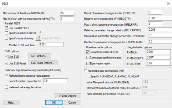
The Parameter Estimation | [[File:PEST ParameterEstimation.png|thumb|550 px|The ''PEST'' parameter estimation dialog]] | ||
The ''PEST'' dialog (''MODFLOW'' | '''Parameter Estimation''') allows the editing of inverse modeling options that are specific to PEST. This dialog is available when ''Parameter Estimation'' option is chosen as the [[GMS:Global Options/Basic Package|''Run'' option]] in the [[GMS:Global Options/Basic Package|''Global Options\Basic Package'']] dialog. | |||
==Max number of iterations (NOPTMAX)== | ==Max number of iterations (NOPTMAX)== | ||
This value (NOPTMAX) sets the maximum number of | This value (NOPTMAX) sets the maximum number of optimization iterations that PEST is permitted to undertake on a particular parameter estimation run. To ensure that PEST termination is triggered by other criteria, more indicative of parameter convergence to an optimal set or of the futility of further processing, set this variable very high. A value of 20 to 30 is often appropriate. | ||
If NOPTMAX is set to 0, PEST will not calculate the Jacobian matrix. Instead it will terminate execution after just one model run. This setting can thus be used when | If NOPTMAX is set to 0, PEST will not calculate the Jacobian matrix. Instead it will terminate execution after just one model run. This setting can thus be used when calculating the objective function corresponding to a particular parameter set and/or to inspect observation residuals corresponding to that parameter set. | ||
If NOPTMAX is set to –1, PEST will terminate execution immediately after it has calculated the Jacobian matrix for the first time. The parameter covariance, correlation coefficient and eigenvector matrices will be written to the run record file, and parameter sensitivities will be written to the sensitivity file; these are based on the initial parameter set supplied in the PEST control file. | If NOPTMAX is set to –1, PEST will terminate execution immediately after it has calculated the Jacobian matrix for the first time. The parameter covariance, correlation coefficient and eigenvector matrices will be written to the run record file, and parameter sensitivities will be written to the sensitivity file; these are based on the initial parameter set supplied in the PEST control file. | ||
| Line 21: | Line 22: | ||
(Φi being the objective function value at the end of the i’th optimisation iteration and Φmin being the lowest objective function achieved to date), PEST will consider that the optimisation process is at an end. | (Φi being the objective function value at the end of the i’th optimisation iteration and Φmin being the lowest objective function achieved to date), PEST will consider that the optimisation process is at an end. | ||
For many cases 4 and 0.01 are suitable values for NPHISTP and PHIREDSTP respectively. However | For many cases 4 and 0.01 are suitable values for NPHISTP and PHIREDSTP respectively. However, be careful not to set NPHISTP too low if the optimal values for some parameters are near or at their upper or lower bounds. In this case it is possible that the magnitude of the parameter upgrade vector may be curtailed over one or a number of optimisation iterations to ensure that no parameter value overshoots its bound. The result may be smaller reductions in the objective function than would otherwise occur. | ||
===Max number of relative parameter change iterations (NRELPAR); Relative parameter change criterion (RELPARSTP)=== | ===Max number of relative parameter change iterations (NRELPAR); Relative parameter change criterion (RELPARSTP)=== | ||
If the magnitude of the maximum relative parameter change between optimisation iterations is less than the Relative Parameter Change Criterion (RELPARSTP) over Max # of Relative Parameter Change | If the magnitude of the maximum relative parameter change between optimisation iterations is less than the ''Relative Parameter Change Criterion (RELPARSTP)'' over ''Max # of Relative Parameter Change Iteration (NRELPAR)'' successive iterations, PEST will cease execution. | ||
All adjustable parameters, whether they are relative-limited or factor-limited, are involved in the calculation of the maximum relative parameter change. RELPARSTP is a real variable for which a value of 0.01 is often suitable. NRELPAR is an integer variable; a value of 2 or 3 is normally satisfactory. | All adjustable parameters, whether they are relative-limited or factor-limited, are involved in the calculation of the maximum relative parameter change. RELPARSTP is a real variable for which a value of 0.01 is often suitable. NRELPAR is an integer variable; a value of 2 or 3 is normally satisfactory. | ||
Max relative parameter change per iteration | ===Max relative parameter change per iteration=== | ||
This (RELPARMAX) is the maximum relative change that a parameter is allowed to undergo between optimisation iterations. | This (RELPARMAX) is the maximum relative change that a parameter is allowed to undergo between optimisation iterations. | ||
| Line 35: | Line 36: | ||
===Run-time matrix options=== | ===Run-time matrix options=== | ||
Select these options if | Select these options if wanting these arrays written to external files. These arrays will also be written to the PEST output file (*.rec). | ||
===Measurement obj func upper limit (PHIMLIM)=== | ===Measurement obj func upper limit (PHIMLIM)=== | ||
| Line 43: | Line 44: | ||
This is the acceptable level for the measurement objective function that PEST uses to change its method of calculating the Marquardt Lamdas (see PEST documentation). | This is the acceptable level for the measurement objective function that PEST uses to change its method of calculating the Marquardt Lamdas (see PEST documentation). | ||
Normally PHIMACCEPT should be about 5% to 10% greater than PHIMLIM. However if PEST is performing well, | Normally PHIMACCEPT should be about 5% to 10% greater than PHIMLIM. However if PEST is performing well, the user may wish to make it closer to PHIMLIM than this. In choosing the best parameter set at any stage of the optimisation process (for recording in the parameter value file) PEST looks at all parameter sets for which it has carried out model runs up to that point in the process. If any of these runs have resulted in an objective function less than PHIMACCEPT, it then searches from among these runs for the parameter set which gave rise to the lowest regularisation objective function. If PHIMACCEPT is set too close to PHIMLIM, PEST’s selection of the best parameter set may be restricted somewhat, for there may be some parameter sets for which the measurement objective function Φm is just above PHIMACCEPT but for which Φr is quite low. Alternatively, if PHIMACCEPT is set too large, then PEST might not try hard enough to reduce Φm to Φmi, preferring instead to work within the weaker constraint set by PHIMACCEPT. When working in regularisation mode, PEST prints out Φr and Φm for every parameter upgrade attempt. It will be apparent from this information whether PHIMACCEPT has been set correctly. | ||
===FRACPHIM=== | ===FRACPHIM=== | ||
PEST ignores the value supplied for FRACPHIM unless it is greater than zero. A value of between zero and 1.0 (but normally less than about 0.3) can be supplied for this variable if | PEST ignores the value supplied for FRACPHIM unless it is greater than zero. A value of between zero and 1.0 (but normally less than about 0.3) can be supplied for this variable if the user is unsure what value to use for PHIMLIM. See the PEST documentation. | ||
===Automatic user intervention (AUI)=== | ===Automatic user intervention (AUI)=== | ||
| Line 54: | Line 55: | ||
==Parallel PEST== | ==Parallel PEST== | ||
GMS allows | GMS allows running PEST in parallel on a single machine to take advantage of multiple cores with the Parallel PEST Utility. This can greatly speed up the PEST runs. | ||
* | *''Specify number of slaves'' | ||
*:"Slaves" refers to the separate processes that will be run in parallel. | *:"Slaves" refers to the separate processes that will be run in parallel. Specify the number of slaves or, if not specified, GMS will automatically determine the number of cores available on the machine and use that for the number of slaves. | ||
* | *''Specify slave directory'' | ||
*:The wait time is the amount of time that PEST will pause at certain strategic places in their communication. Normally the default value should work fine. However, if either PEST reports a sharing violation on | *:By default, GMS uses the system temp directory as the slave directory. However, a user may specify a different folder for the files that are used by the slaves. If the specified slave directory is invalid then GMS will use the system temp directory. | ||
*''Parallel PEST wait time'' | |||
*:The wait time is the amount of time that PEST will pause at certain strategic places in their communication. Normally the default value should work fine. However, if either PEST reports a sharing violation on the hard drive then increase the value of the wait time. | |||
The PEST model can also be run with parallel processing across multiple machines with setup outside of GMS with PSLAVE. More information about Parallel PEST can be found in the [http://www.pesthomepage.org/getfiles.php?file=newpestman1.pdf PEST Manual] starting on page 222 from the [http://www.pesthomepage.org/Downloads.php PEST Downloads page]. | |||
==SVD (Singular Value Decomposition)== | ==SVD (Singular Value Decomposition)== | ||
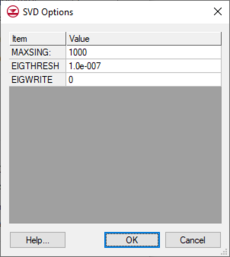
[[File:SVD Options.png|thumb|230 px|The ''SVD Options'' dialog]] | |||
The ''Use SVD'' toggle is available to turn on the SVD functionality in PEST. For a more complete explanation of SVD, see the [http://gmsdocs.aquaveo.com/pest.pdf PEST manual] in section 8.4. The inputs to the SVD process can be edited by selecting the '''SVD Options''' button. | The ''Use SVD'' toggle is available to turn on the SVD functionality in PEST. For a more complete explanation of SVD, see the [http://gmsdocs.aquaveo.com/pest.pdf PEST manual] in section 8.4. The inputs to the SVD process can be edited by selecting the '''SVD Options''' button. | ||
| Line 71: | Line 76: | ||
==SVD-Assist== | ==SVD-Assist== | ||
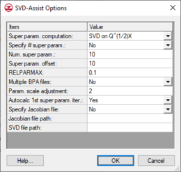
[[File:SVD-Assist Options.png|thumb|260 px|The ''SVD-Assist Options'' dialog]] | |||
The | The ''Use SVD-Assist'' toggle turns on the SVD-Assist process for PEST. This process is particularly advantageous for models that have hundreds or thousands of parameters (such as pilot points). SVD-Assist involves 3 basic steps. | ||
#First, PEST runs MODFLOW once for every parameter in order to compute a matrix. This information is used to create super parameters that are combinations of the parameters originally specified. | #First, PEST runs MODFLOW once for every parameter in order to compute a matrix. This information is used to create super parameters that are combinations of the parameters originally specified. | ||
#Second, SVDAPREP is run to create a new PEST control file. The options for SVDAPREP are entered by selecting the '''SVD-Assist Options''' button. For more information on each of these options see the PEST manual in section 8.5.4.2. The most important option entered is the ''Specify # super param'' and this is set to | #Second, SVDAPREP is run to create a new PEST control file. The options for SVDAPREP are entered by selecting the '''SVD-Assist Options''' button. For more information on each of these options see the PEST manual in section 8.5.4.2. The most important option entered is the ''Specify # super param'' and this is set to ''No'' by default. When this option is set to ''No'', then the information written to the *.svd file will be used to specify the number of super parameters. | ||
#Third, PEST runs using the new control file written by SVDAPREP. This should result in significantly fewer model runs for each PEST iteration. This often results in an order of magnitude reduction in the number of runs required for each PEST iteration. | #Third, PEST runs using the new control file written by SVDAPREP. This should result in significantly fewer model runs for each PEST iteration. This often results in an order of magnitude reduction in the number of runs required for each PEST iteration. | ||
:'''''Note:''''' When PEST runs with SVD-Assist, it does not output sensitivities of individual parameters. Therefore there is not an option to view parameters a parameters sensitivity plot. | |||
==Tikhonov Regularization== | ==Tikhonov Regularization== | ||
Tikhonov Regularization (prior information for pilot points). This section of the dialog allows the user to select the method for include Tikhonov regularization in the PEST run. If neither option is turned on then regularization will not be included in the PEST run. | Tikhonov Regularization (prior information for pilot points). This section of the dialog allows the user to select the method for include Tikhonov regularization in the PEST run. If neither option is turned on then regularization will not be included in the PEST run. | ||
The first option, Preferred homogeneous regularization, is the option that GMS has always supported with pilot points. When using this option, prior information equations are included that impose a homogeneity constraint on the pilot points. This means that in absence of other information, pilot points that are near to one another should have about the same value. | The first option, ''Preferred homogeneous regularization'', is the option that GMS has always supported with pilot points. When using this option, prior information equations are included that impose a homogeneity constraint on the pilot points. This means that in absence of other information, pilot points that are near to one another should have about the same value. | ||
*Prior information power factor | *Prior information power factor | ||
*:This is used to change the weight applied to the prior information equations for the pilot points. A value of 1 is normally sufficient. The prior information equations impose a homogeneity constraint on the pilot points. This means that in absence of other information, pilot points that are near to one another should have about the same value. When the prior information equations are created GMS will compute an inverse distance weight between each pilot point and all other pilot points for a given parameter. This weight is then raised to the power of the ''Prior information power factor'' and assigned to the equation for a given pair of points. So to increase the homogeneity constraint (assign a higher weight to the prior information equation), the user should decrease this value. To decrease the homogeneity constraint (assign a lower weight to the prior information equation), the user should increase this value. | *:This is used to change the weight applied to the prior information equations for the pilot points. A value of 1 is normally sufficient. The prior information equations impose a homogeneity constraint on the pilot points. This means that in absence of other information, pilot points that are near to one another should have about the same value. When the prior information equations are created GMS will compute an inverse distance weight between each pilot point and all other pilot points for a given parameter. This weight is then raised to the power of the ''Prior information power factor'' and assigned to the equation for a given pair of points. So to increase the homogeneity constraint (assign a higher weight to the prior information equation), the user should decrease this value. To decrease the homogeneity constraint (assign a lower weight to the prior information equation), the user should increase this value. | ||
The second option, Preferred value regularization, is a new option beginning with GMS version 8.0. When this option is used, prior information equations are included that constrain the pilot points near their starting values. Using this option the user can give a set of starting values to the pilot points based on field data or professional judgment. PEST will only change those values if necessary to calibrate the model. | The second option, ''Preferred value regularization'', is a new option beginning with GMS version 8.0. When this option is used, prior information equations are included that constrain the pilot points near their starting values. Using this option the user can give a set of starting values to the pilot points based on field data or professional judgment. PEST will only change those values if necessary to calibrate the model. | ||
Also new in GMS 8.0, parameters of different types (HK, RCH) are put into different regularization groups. According to John Doherty, this helps differentiate weighting amongst pertinent prior information equations. | Also new in GMS 8.0, parameters of different types (HK, RCH) are put into different regularization groups. According to John Doherty, this helps differentiate weighting amongst pertinent prior information equations. | ||
| Line 92: | Line 99: | ||
==See also== | ==See also== | ||
[[GMS:Model Calibration|Model Calibration]] | *[[GMS:Model Calibration|Model Calibration]] | ||
{{Navbox GMS}} | {{Navbox GMS}} | ||
[[Category:MODFLOW]] | [[Category:MODFLOW]] | ||
[[Category:Calibration]] | [[Category:Calibration]] | ||
[[Category:Calibration Dialogs]] | |||
[[Category:MODFLOW Dialogs|P]] | |||
[[Category:PEST|Dialog]] | |||
[[Category:Needs Update]] | |||


