GMS:Risk Analysis Wizard
| MODFLOW | |
|---|---|
| Pre-processing | |
| MODFLOW Commands | |
| Building a MODFLOW Model | |
| Map to MODFLOW | |
| Calibration | |
| Packages Supported in GMS | |
| Saving a MODFLOW Simulation | |
| Importing MODFLOW Files | |
| Unsupported MODFLOW Features | |
| Run MODFLOW | |
| Post-processing | |
| MODFLOW Display Options | |
| MODFLOW Post-Processing Viewing Options | |
| Reading a MODFLOW Simulation | |
| Tutorials | |
| Packages | |
| Flow: | BCF6, HUF, LPF, UPW |
| Solvers: | SMS |
| Other: | UZF1 |
The Risk Analysis Wizard is a tool for refining stochastic modeling results. The Risk Analysis Wizard has two options. The user can either perform a Capture Zone Analysis or a Threshold Analysis. Capture zone analysis requires a MODFLOW solution set, but threshold analysis can be performed on any solution set type.
Contents
Capture Zone Analysis
Capture zone analysis includes running MODPATH for each of the MODFLOW solutions to generate a capture zone for each well or zone code group in the MODFLOW model. These capture zones are combined into one probabilistic capture zone
Threshold Analysis
Threshold analysis is similar to capture zone analysis, but threshold analysis can be performed using any type of 3D dataset that has been read into the Project Explorer.
- First select a simulation set from the Project Explorer.
- Next, set up rules for generating a probabilistic threshold dataset.
For example, the user might be looking at a specific contaminant and want to know what the probability is that the concentration of this contaminant will be above the EPA level for drinking water. The user would generate a rule reflecting this limit. After processing all rules for each simulation, GMS creates a probabilistic threshold dataset.
Risk Analysis Wizard Dialogs
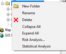
The Risk Analysis Wizard is entered through the right-click menu for a folder in the Project Explorer and choose Risk Analysis... .
Choosing Between Capture Zone and Threshold Analysis
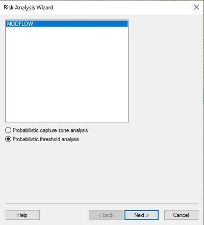
The first step in the Risk Analysis Wizard is to choose what type of simulations to process.
The window will list all the solution types as the analysis wizard will only process solutions of the same type. Probabilistic capture zone analysis can only be performed on MODFLOW solutions. Probabilistic threshold analysis can be performed on any solution type.
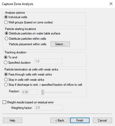
Capture Zone Analysis Dialog
Capture Zone Analysis can only be performed on MODFLOW solutions
Analysis Options – Individual wells
- Choose this option to create a probabilistic capture zone for each uniquely named well in the MODFLOW model.
Analysis Options – Well groups
- Choose this option to create a probabilistic capture zone for each different zone code number.
Particle Starting Locations – Distribute particles on water table surface
- Choose this option to distribute particles only on the water table surface. By default, one particle is placed at the xy center of the cell at the water table, but the user can use the Particle placement within cells option to change the number of particles placed on the water table in each cell. This option will create a 2D probabilistic capture zone representing the intersection of the entire 3D probabilistic capture zone with the water table.
Particle Starting Locations – Distribute particles within cells
- Choose this option to distribute particles within each cell. By default, one particle is placed at the center of each cell, but the user can use the Particle placement within cells option to change the number of particles placed on within each cell. This option creates three different probabilistic capture zones. The first represents the 3D capture zone, the other two represent different 2D projections of the 3D capture zone.
Tracking Duration – To end
- This option sets MODPATH to move particles through the flow field until they exit the model.
Tracking Duration – Specified duration
- This option sets MODPATH to move particles through the flow field until they either exit the model or the time reaches the duration set, which ever comes first.
Particle Placement Within Cells'
- This option allows the user to change the number of particles per cell from the default of one. Increase the number of particles leads to a smoother capture zone, but drastically increases the computation time.
Weight Results Based On Residual Error
- In all of the capture zone methods, the algorithms used to synthesize the probability data set can be weighted using observation data. This makes it possible to give more weight to model instances with smaller calibration error when calculating the capture zone probabilities. The weighted head and flow observations can be compared to the computed values to come up with a global error norm, E, for each model run. This error norm can be based on the root mean squared (RMS) error, the sum of the squared weighted residuals, or any other measure selected by the modeler. For capture zone analysis, GMS uses the sum of squared weighted residuals (SSWR) for the error norm. The error norm from each MODFLOW run is used to compute a weight for the given solution using the following equation:
- Where Wi is the weight applied to solution i, α is a user-defined factor, ME is the mean of the error values from all solutions, Ejk is the error for solution i, and SD is the standard deviation of error values from all solutions. The weights are also normalized as follows
- so that the weights sum to unity. Equation 1 was developed to give the greater emphasis to the lower error values and to allow controlling the relative emphasis given to low vs. high values simply by adjusting the α value. The equation also avoids problems when one of the error values is zero, since a zero error value does not result in an infinite weight. The equation is also designed to allow scaling the weights according to the data being examined. This is done by subtracting the individual SSWR from the mean error and dividing by the standard deviation.
- Equation 1 centers the weights on the mean error. The relative weight given to values differing from the mean is biased by the factor. This makes it possible to bias the resulting weight using knowledge of the site and the quality of the observation data.
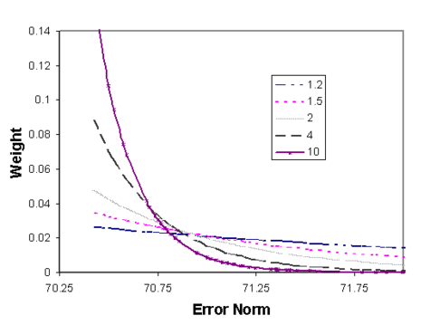
- The figure below shows how the α factor in Equation 1 affects the weight applied to a given error. An α factor of 1.2 makes the contribution of each SSWR almost linear, whereas an α factor of ten gives most of the weight to the lowest 5–10 percent while discounting the other error values. Typically use an α value of 2.0.
Threshold Analysis Dialog
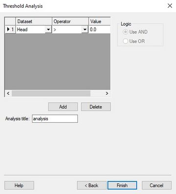
Threshold analysis can be performed on any collection of 3D datasets. The threshold analysis dataset is created by using rules. For each rule, select a dataset (only applies to solutions with multiple data sets.), the greater or less than sign and a value. There is no limit to the number of rulse that can be created. The AND and OR logic options allow the user to use: 1st rule AND 2nd rule AND 3rd rule; or 1st rule OR 2nd rule OR 3rd rule. Threshold analysis creates one 3D dataset.
| GMS – Groundwater Modeling System | ||
|---|---|---|
| Modules: | 2D Grid • 2D Mesh • 2D Scatter Point • 3D Grid • 3D Mesh • 3D Scatter Point • Boreholes • GIS • Map • Solid • TINs • UGrids | |
| Models: | FEFLOW • FEMWATER • HydroGeoSphere • MODAEM • MODFLOW • MODPATH • mod-PATH3DU • MT3DMS • MT3D-USGS • PEST • PHT3D • RT3D • SEAM3D • SEAWAT • SEEP2D • T-PROGS • ZONEBUDGET | |
| Aquaveo | ||
