GMS:Model Calibration: Difference between revisions
From XMS Wiki
Jump to navigationJump to search
(Added introductory explanatory paragraph) |
No edit summary |
||
| Line 4: | Line 4: | ||
An important part of any groundwater modeling exercise is the model calibration process. In order for a groundwater model to be used in any type of predictive role, it must be demonstrated that the model can successfully simulate observed aquifer behavior. Calibration is a process wherein certain parameters of the model such as recharge and hydraulic conductivity are altered in a systematic fashion and the model is repeatedly run until the computed solution matches field-observed values within an acceptable level of accuracy. | An important part of any groundwater modeling exercise is the model calibration process. In order for a groundwater model to be used in any type of predictive role, it must be demonstrated that the model can successfully simulate observed aquifer behavior. Calibration is a process wherein certain parameters of the model such as recharge and hydraulic conductivity are altered in a systematic fashion and the model is repeatedly run until the computed solution matches field-observed values within an acceptable level of accuracy. | ||
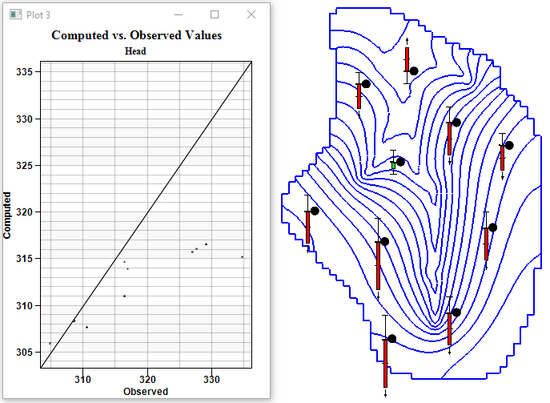
Calibration is the process of modifying the input parameters to a groundwater model until the output from the model matches an observed set of data. GMS includes a suite of tools to assist in the process of calibrating a groundwater model. Both point and flux observations are supported. When a computed solution is imported to GMS, the point and flux residual errors are plotted on a set of [[GMS:Calibration_Targets|calibration targets]] and a variety of plots can be generated showing overall calibration statistics. Most of the calibration tools can be used with any of the models in GMS. [[GMS:Automated Parameter Estimation|Automated | Calibration is the process of modifying the input parameters to a groundwater model until the output from the model matches an observed set of data. GMS includes a suite of tools to assist in the process of calibrating a groundwater model. Both point and flux observations are supported. When a computed solution is imported to GMS, the point and flux residual errors are plotted on a set of [[GMS:Calibration_Targets|calibration targets]] and a variety of plots can be generated showing overall calibration statistics. Most of the calibration tools can be used with any of the models in GMS. [[GMS:Automated Parameter Estimation|Automated parameter estimation]] is supported for [[GMS:MODFLOW|MODFLOW]] models via [[GMS:PEST|PEST]]. | ||
Two types of [[GMS:Observations|observations]] can be defined in GMS: [[GMS:Observations#Point_Observations|point observations]] and [[GMS:Observations#Flow_Observations|flow observations]]. Both types of observations are defined in the [[GMS:Map_Module| | Two types of [[GMS:Observations|observations]] can be defined in GMS: [[GMS:Observations#Point_Observations|point observations]] and [[GMS:Observations#Flow_Observations|flow observations]]. Both types of observations are defined in the [[GMS:Map_Module|Map module]] and are associated with [[GMS:Feature_Objects|points, arcs, and polygons]]. Point observations represent locations in the field where some value has been observed. In most cases, the points will correspond to observation wells and the value will be the elevation of the groundwater table (the head). Flow observations represent linear or areal objects such as streams and reservoirs where the gain or loss between the aquifer and the object has been measured or estimated. Both point and flow observations can be assigned a confidence interval or calibration target. While point observations can be used with any model, flow observations can only be used with MODFLOW. | ||
Once a set of observed point and flow values has been entered, each time a model solution is imported, GMS automatically interpolates the computed solution to the observation points. For some models ([[GMS:MODFLOW|MODFLOW]]) the model outputs the computed values at the observation points. Also, MODFLOW outputs the computed flow for the flow observations. A calibration target representing the magnitude of the residual error is displayed next to each observation point and each flow object as shown below. The residual is calculated as the observed value minus the simulated value which matches MODFLOW. The size of the target is based on the confidence interval or the standard deviation. In addition to the calibration targets next to the observation points, a user can choose to display any of a number of statistical [[GMS:Plot_Wizard|plots]]. | Once a set of observed point and flow values has been entered, each time a model solution is imported, GMS automatically interpolates the computed solution to the observation points. For some models ([[GMS:MODFLOW|MODFLOW]]) the model outputs the computed values at the observation points. Also, MODFLOW outputs the computed flow for the flow observations. A calibration target representing the magnitude of the residual error is displayed next to each observation point and each flow object as shown below. The residual is calculated as the observed value minus the simulated value which matches MODFLOW. The size of the target is based on the confidence interval or the standard deviation. In addition to the calibration targets next to the observation points, a user can choose to display any of a number of statistical [[GMS:Plot_Wizard|plots]]. | ||
